Practical aspects of Deep Learning

---

Regularization

What we learn in Week 3 is L2 Regularization.

L1 Regularization is without the square of the $\theta$.

Implementation tip: if you implement gradient descent, one of the steps to debug gradient descent is to plot the cost function J as a function of the number of iterations of gradient descent and you want to see that the cost function J decreases monotonically after every elevation of gradient descent with regularization. If you plot the old definition of J (no regularization) then you might not see it decrease monotonically.

---

Dropout Regularization

For reducing overfitting

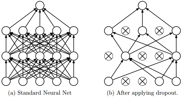
Implementing Dropout (illustrate with l = 3, and keep-prob = 0.8):

d3 = np.random.rand(a3.shape[0], a3.shape[1]) < keep-prob
a3 = np.multiple(a3, d3)
a3 /= keep-prob

One big downside of drop out is that the cost function J is no longer well-defined. J is not going downhill on very iteration.

Many of the first successful implementations of drop outs were to computer vision. So in computer vision, the input size is so big, inputting all these pixels that you almost never have enough data. And so drop out is very frequently used by computer vision

Note: Dropout doesn’t work with gradient checking because J is not consistent. You can first turn off dropout (set keep_prob = 1.0), run gradient checking and then turn on dropout again.

---

Other regularization methods

• Data augmentation
  • For example in a computer vision data:
    • You can flip all your pictures horizontally this will give you m more data instances.
    • You could also apply a random position and rotation to an image to get more data.
  • For example in OCR, you can impose random rotations and distortions to digits/letters.
  • New data obtained using this technique isn’t as good as the real independent data, but still can be used as a regularization technique.
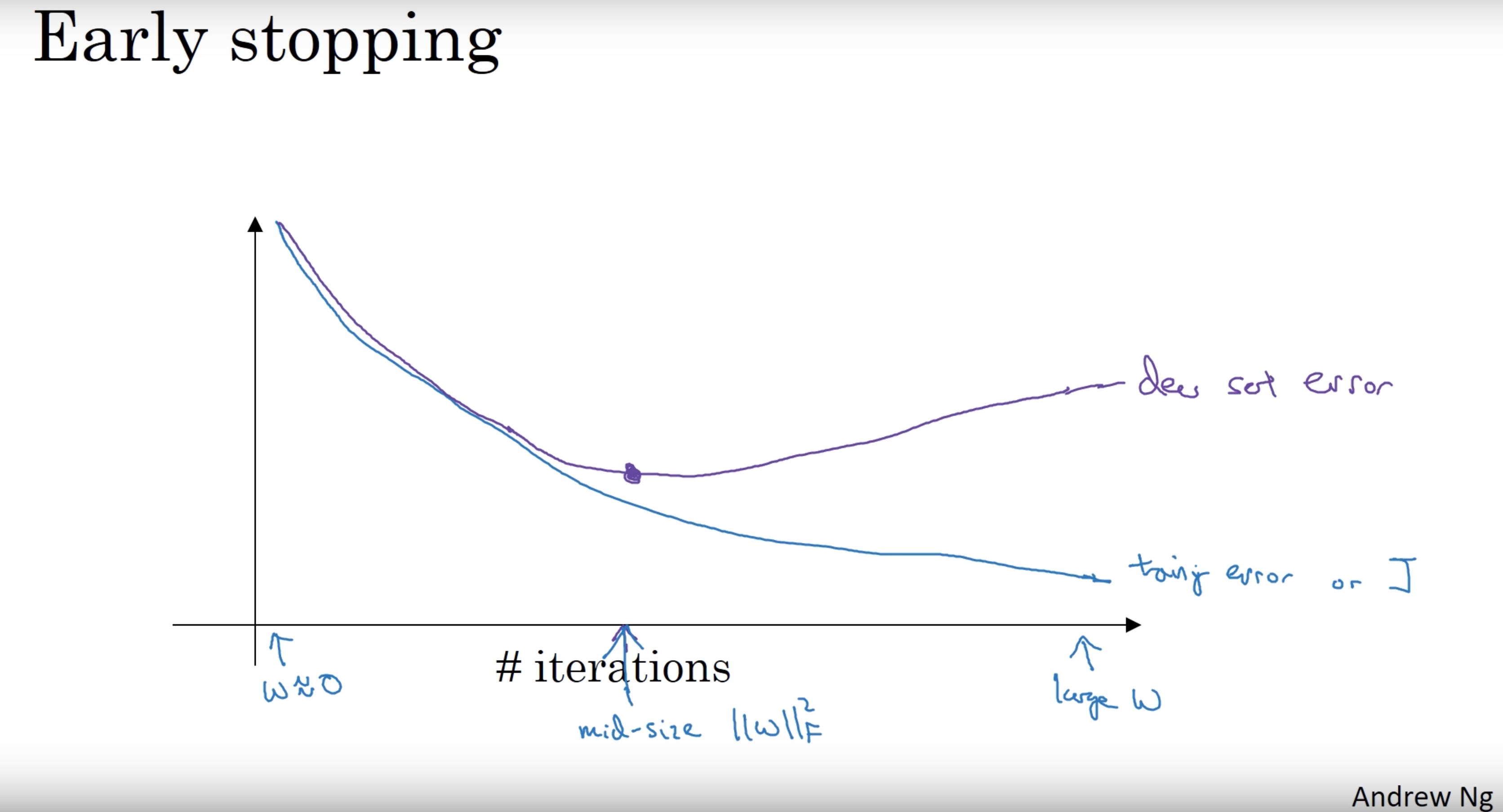
• Early stopping
  • In this technique we plot the training set and the dev set cost together for each iteration. At some iteration the dev set cost will stop decreasing and will start increasing.
  • We will pick the point at which the training set error and dev set error are best (lowest training cost with lowest dev cost).
  • We will take these parameters as the best parameters.

---

Vanishing / Exploding Gradient

The level number of deep learning network layers can be large. So if the Ws are just a little bit bigger than one or just a little bit bigger than the identity matrix, then with a very deep network the activations can explode. (i.e. W .^ 100)

And if W is just a little bit less than identity. The activations will decrease exponentially

---

Weight Initialization

A partial solution to the Vanishing / Exploding gradients in NN is better or more careful choice of the random initialization of weights

So, we need the variance which equals $\frac{1}{n_x}$ to be the range of W’s

Here are three ways to weight initailize $W$:

1. For $tanh$ activation: np.random.rand(shape) * np.sqrt(1/n[l-1])
2. For ReLU: np.random.rand(shape) * np.sqrt(2/n[l-1])
3. Xavier Initialization: np.random.rand(shape) * np.sqrt(2/(n[l-1] + n[l]))

---

Gradient checking

$$ \begin{align} \dfrac{\partial}{\partial\Theta}J(\Theta) \approx \dfrac{J(\Theta + \epsilon) - J(\Theta - \epsilon)}{2\epsilon} \end{align} $$

$$ difference = \frac {\mid\mid grad - gradapprox \mid\mid_2}{\mid\mid grad \mid\mid_2 + \mid\mid gradapprox \mid\mid_2}$$ with $\epsilon = 10^{-7}$ (|| - Euclidean vector norm):

• if it is $< 10^{-7}$ - great, very likely the backpropagation implementation is correct
• if around $10^{-5}$ - can be OK, but need to inspect if there are no particularly big values in $gradapprox - grad$
• if it is $\geq 10^{-3}$ - bad, probably there is a bug in backpropagation implementation

---

Optimization Algorithms

---

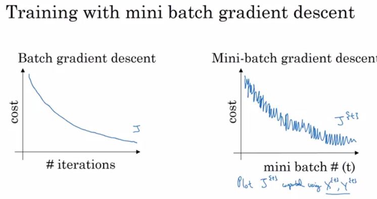
Mini-batch Gradient Descent

In Batch gradient descent we run the gradient descent on the whole dataset.

While in Mini-Batch gradient descent we run the gradient descent on the mini datasets.

Training NN with a large data is slow. So we break the data set into mini batches for both $X$ and $Y$ ==> $t: X^{\{t\}}, Y^{\{t\}}$

Pseudo code:

for t = 1:num_of_batches                         # this is called an epoch
	AL, caches = forward_prop(X{t}, Y{t})
	cost = compute_cost(AL, Y{t})
	grads = backward_prop(AL, caches)
	update_parameters(grads)

Mini-batch size:

• (mini batch size = m) ==> Batch gradient descent
  1. Too long per iteration (epoch)
• (mini batch size = 1) ==> Stochastic gradient descent (SGD)
  1. Too noisy regarding cost minimization (can be reduced by using smaller learning rate)
  2. Don’t ever converge (oscelates a lot around the minimum cost)
  3. Lose speedup from vectorization
• (mini batch size = between 1 and m) ==> Mini-batch gradient descent
  1. Faster learning:
     • Have the vectorization advantage
     • make progress without waiting to process the entire training set
  2. Doesn’t always exactly converge (oscelates in a very small region, but you can reduce learning rate)

Guidelines for choosing mini-batch size

1. If small training set (< 2000 examples) - use batch gradient descent.
2. It has to be a power of 2 (because of the way computer memory is layed out and accessed, sometimes your code runs faster if your mini-batch size is a power of 2): 64, 128, 256, 512, 1024, …
3. Make sure that mini-batch fits in CPU/GPU memory.
4. Mini-batch size is a hyperparameter.

---

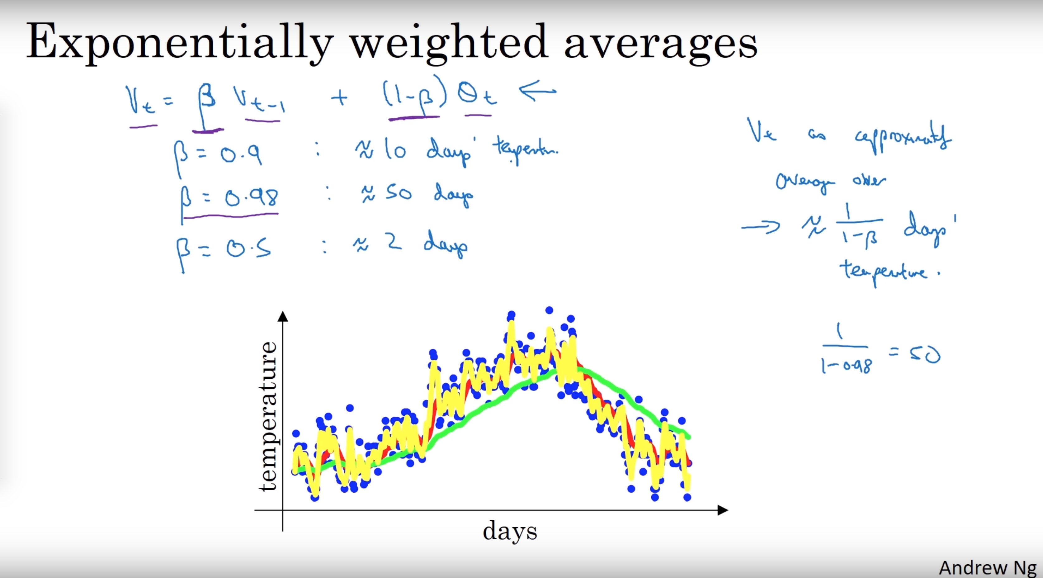
Exponentially Weighted Averages

There are optimization algorithms that are better than gradient descent, but you should first learn about Exponentially weighted averages.

$V_t$ is the weighted average for entry t, and $\theta_t$ is the value for entry t $$ V_t = \beta V_{t-1} + (1 - \beta) \theta_t $$

If we plot this it will represent averages over $\frac{1}{1 - \beta}$ entries:

• $\beta = 0.9$ will average last 10 entries
• $\beta = 0.98$ will average last 50 entries
• $\beta = 0.5$ will average last 2 entries

Intuition:

• Increase $\beta$, the shift the curve slightly to the right.
• Decreasing $\beta$ will create more oscillation within the curve.

Bias correction in exponentially weighted averages

When $V_0 = 0$, the bias of the weighted averages is shifted and the accuracy suffers at the start

$$ V_t = \frac{\beta V_{t-1} + (1 - \beta) \theta_t}{ 1 - \beta^t } $$

Note: As t becomes larger the $1 - \beta^t$ becomes close to 1

---

Gradient Descent with Momentum

The simple idea is to calculate the exponentially weighted averages for your gradients and then update your weights with the new values.

$$ \begin{align} &v_{dW^{[l]}} = \beta v_{dW^{[l]}} + (1 - \beta) dW^{[l]} \newline &W^{[l]} = W^{[l]} - \alpha v_{dW^{[l]}} \end{align} $$

Momentum helps the cost function to go to the minimum point in a more fast and consistent way.

Note: $\beta$ is another hyperparameter. $\beta = 0.9$ is very common and works very well in most cases.

---

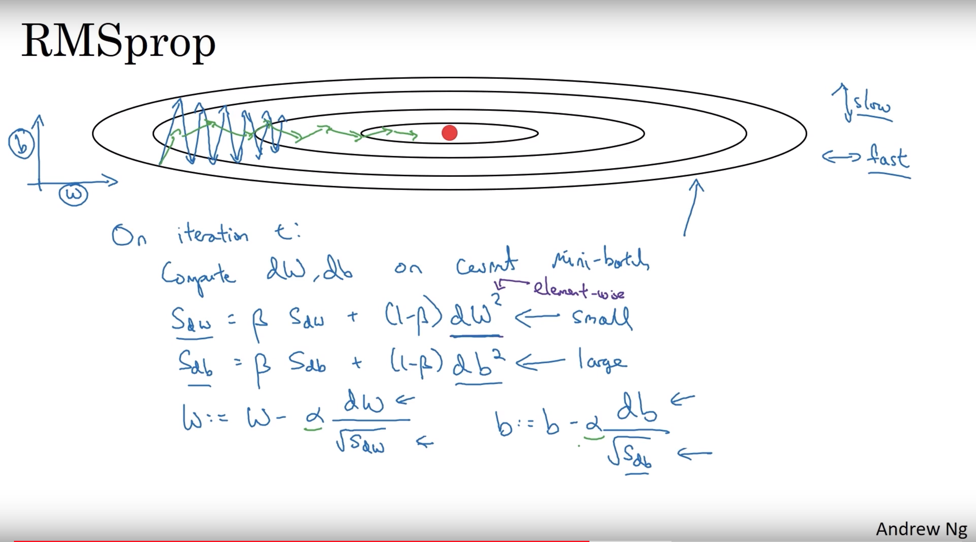
RMSprop

Stands for Root mean square prop.

RMSprop will make the cost function move slower on the vertical direction and faster on the horizontal direction

$$ \begin{align} & s_{dW^{[l]}} = \beta_2 s_{dW^{[l]}} + (1 - \beta_2) (\frac{\partial J }{\partial dW^{[l]} })^2 \newline & W^{[l]} = W^{[l]} - \alpha \frac{dW^{[l]}}{\sqrt{s_{dW^{[l]}}} + \epsilon} \end{align} $$

Notes:

1. Name the beta $\beta_2$ is to differentiate the beta in momentum
2. $\epsilon$ is used to ensure denominator is not zero

---

Adam

Stands for Adaptive Moment Estimation

Simply puts RMSprop and momentum together:

$$ \begin{align} & v_{W^{[l]}} = \beta_1 v_{W^{[l]}} + (1 - \beta_1) \frac{\partial J }{ \partial W^{[l]} } \newline & v^{corrected}_{W^{[l]}} = \frac{v_{W^{[l]}}}{1 - (\beta_1)^t} \newline & s_{W^{[l]}} = \beta_2 s_{W^{[l]}} + (1 - \beta_2) (\frac{\partial J }{\partial W^{[l]} })^2 \newline & s^{corrected}_{W^{[l]}} = \frac{s_{W^{[l]}}}{1 - (\beta_2)^t} \newline & W^{[l]} = W^{[l]} - \alpha \frac{v^{corrected}_{W^{[l]}}}{\sqrt{s^{corrected}_{W^{[l]}}}+\varepsilon} \end{align} $$

Hyperparameters for Adam:

1. Learning rate: needed to be tuned.
2. $\beta_1$: parameter of the momentum - 0.9 is recommended by default.
3. $\beta_2$: parameter of the RMSprop - 0.999 is recommended by default.
4. $\epsilon$: $10^{-8}$ is recommended by default.

---

Learning rate decay

As mentioned before mini-batch gradient descent won’t reach the optimum point (converge). But by making the learning rate decay with iterations it will be much closer to it because the steps (and possible oscillations) near the optimum are smaller.

Three learning rate decay methods:

$$ \begin{align} & \alpha = \frac{1}{1 + \text{decay_rate} * \text{epoch_num}} * \alpha_0 \newline \newline & \alpha = (0.95 ^ {\text{epoch_num}}) * \alpha_0 \newline \newline & \alpha = \frac{k}{\sqrt{\text{epoch_num}}} * \alpha_0 \end{align} $$

---

The problem of local optima

1. The normal local optima is not likely to appear in a dnn because data is usually high dimensional. For point to be a local optima it has to be a local optima for each of the dimensions which is highly unlikely.
2. It’s unlikely to get stuck in a bad local optima in high dimensions, it is much more likely to get to the saddle point rather to the local optima, which is not a problem.
3. Plateaus can make learning slow:
   • Plateau is a region where the derivative is close to zero for a long time.
   • This is where algorithms like momentum, RMSprop or Adam can help.

---

Hyperparameter tuning, Batch Normalization and Programming Frameworks

---

Tuning Process

Hyperparameters are:

1. Learning rate.
2. Momentum beta.
3. Mini-batch size.
4. No. of hidden units.
5. No. of layers.
6. Learning rate decay.
7. Regularization lambda.
8. Activation functions.
9. Adam beta1 & beta2.

Its hard to decide which hyperparameter is the most important in a problem. It depends a lot on your problem.

One of the ways to tune is to sample a grid with N hyperparameter settings and then try all settings combinations on your problem.

Try random values: don’t use a grid. You can use Coarse to fine sampling scheme:

When you find some hyperparameters values that give you a better performance - zoom into a smaller region around these values and sample more densely within this space.

These methods can be automated.

---

Appropriate Scale

Let’s say you have a specific range for a hyperparameter from “a” to “b” It’s better to search for the right ones using the logarithmic scale rather then in linear scale:

• Calculate: a_log = log(a) # e.g. a = 0.0001 then a_log = -4
• Calculate: b_log = log(b) # e.g. b = 1 then b_log = 0

• Then:

  r = (a_log - b_log) * np.random.rand() + b_log
  # In the example the range would be from [-4, 0] because rand range [0,1)
  result = 10^r
  

For example, if we want to use the last method on exploring on the “momentum beta”: * Beta best range is from 0.9 to 0.999. * You should search for 1 - beta in range 0.001 to 0.1 (1 - 0.9 and 1 - 0.999) and the use a = 0.001 and b = 0.1. Then:

a_log = -3
b_log = -1
r = (a_log - b_log) * np.random.rand() + b_log
beta = 1 - 10^r   # because 1 - beta = 10^r

• The reason why randomize $1-\beta$ instead of $\beta$ is because $\frac{1}{1-\beta}$ is too sensitive when $\beta$ approches to 1

---

Pandas vs. Caviar

1. If you don’t have much computational resources you can use the “babysitting model”. Like Pandas:
   • Day 0 you might initialize your parameter as random and then start training.
   • Then you watch your learning curve gradually decrease over the day.
   • And each day you nudge your parameters a little during training.
2. If you have enough computational resources, you can run some models in parallel and at the end of the day(s) you check the results. Like Caviar.

---

Normalizing Activations In A Network

Batch normalization speeds up learning.

For any hidden layer, we can normalize $A^{[L]}$ to train $W^{[L]} \ b^{[L]}$ faster. In practice, normalizing $Z^{[L]}$ before activation.

Algorithm:

$$ \begin{align} & \mu = \frac{1}{m} \sum_{i}^m Z{[i]} \newline & \sigma^2 = \frac{1}{m} \sum_{i}^m (Z^{[i]} - \mu)^2 \newline & Z_{norm}^{[i]} = \frac{Z^{[i]} - \mu}{\sqrt{\sigma^2 + \epsilon}} \newline & \tilde{Z}^{[i]} = \gamma Z_{norm}^{[i]} + \beta \end{align} $$

Notes:

• $Z_{norm}^{[i]} $ forces the inputs to a distribution with zero mean and variance of 1.
• $\tilde{Z}^{[i]}$ is to make inputs belong to other distribution (with other mean and variance)
• $\gamma$ and $\beta$ are learnable parameters, making the NN learn the distribution of the outputs.
• If $\gamma = \sqrt{\sigma^2 + \epsilon}$ and $\beta = \mu$ then $\tilde{Z}^{[i]} = Z_{norm}^{[i]}$

Why does Batch normalization work?

• The first reason is the same reason as why we normalize X.
• The second reason is that batch normalization reduces the problem of input values changing (shifting).
• Batch normalization does some regularization:
  • Each mini batch is scaled by the mean/variance computed of that mini-batch.
  • This adds some noise to the values Z[l] within that mini batch. So similar to dropout it adds some noise to each hidden layer’s activations.
  • This has a slight regularization effect.
  • Using bigger size of the mini-batch you are reducing noise and therefore regularization effect.
  • Don’t rely on batch normalization as a regularization. It’s intended for normalization of hidden units, activations and therefore speeding up learning. For regularization use other regularization techniques (L2 or dropout).

---

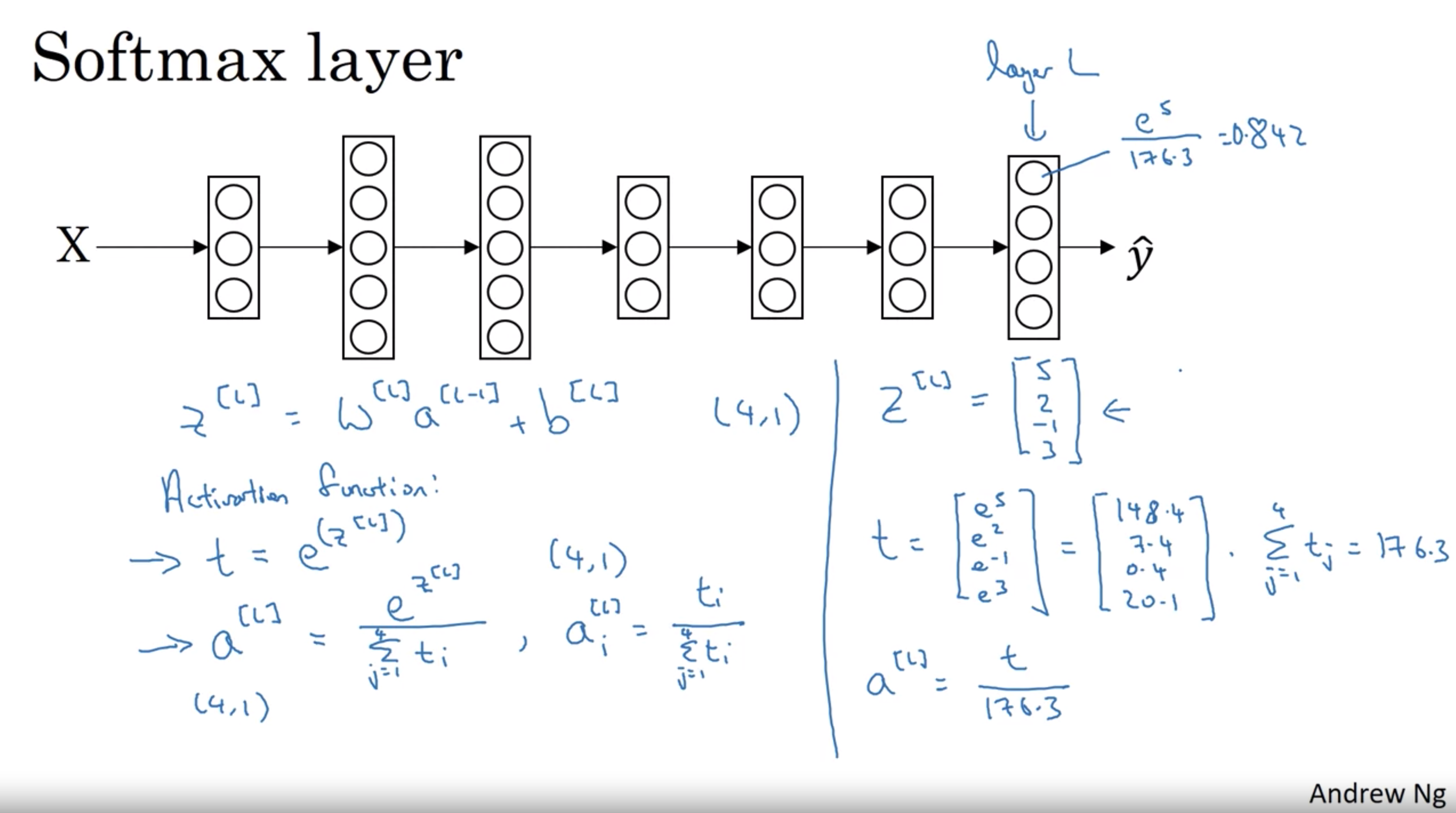
Softmax Regression

Used for multiclass classification/regression.

It is a function that takes as input a vector of K real numbers, and normalizes it into a probability distribution consisting of K probabilities.

We activate softmax regression activation function in the last layer instead of the sigmoid activation.

$$ S_i = \frac{e^{Z_i^{[L]}}}{\sum_{i=i}^K e^{Z_j^{[L]}}} \text{ for } i = 1, \ …, \ K $$

Training a Softmax classifier

$$ \begin{align} & L(y, \hat{y}) = - \sum_{j=1}^K y_j \log{\hat{y_j}} \newline \newline & J(W, b) = - \frac{1}{m} \sum_{i=1}^m L(y_i, \hat{y}_i) \newline \newline & dZ^{[L]} = \hat{Y} - Y \newline \newline & DS_i = \hat{Y} (1 - \hat{Y}) \end{align} $$